LS Geometry Summary

This note is intended to briefly explain three key ideas of our approach in Identifying the latent space geometry of network models through analysis of curvature. These three ideas are

• Embeddability of points via eigenvalues
• Constructing confidence intervals for eigenvalues using bootstrapping.
• Constructing a distance matrix from the graph.

Last updated on February 18, 2021. Please send comments or questions to sl223@uw.edu.

Is there code?

Yes! Check out the github repo here.

Introduction

The latent space (LS) model, originally proposed in Hoff (2002), uses low-dimensional representations of nodes to depict complex, high-dimensional dependencies between nodes in a network. We consider the following generative model.

\[P(g_{ij} = 1 | \nu, z) = \exp(\nu_i + \nu_j - d_{\mathcal{M}}(z_i, z_j))\]

where \(\{\nu_i\}\) are the node-specific propensity to form edges, \(\{z_i\}\) are the latent space locations of the nodes, and \(d_{\mathcal{M}^p(\kappa)}(z_i, z_j)\) is the distance along the surface of \(\mathcal{M}^p(\kappa)\). Our goal is to answer: “Given \(g\) drawn from the LS model, can we estimate the geometry type, dimension, and curvature of \(\mathcal{M}^p(\kappa)\)?’’

Embedding Approach

To motivate our approach, we consider a related problem. Suppose we observe a \(K \times K\) matrix \(D\) that contains the pairwise distances between \(K\) unknown points on \(\mathbb{R}^2\). For example, set \(K = 3\) and let \(D\) take the form

\[D = \begin{pmatrix} 0 & 1 & 2 \\ 1 & 0 & \sqrt{5} \\ 2 & \sqrt{5} & 0 \end{pmatrix} \;.\]

These distances correspond to three points at (0, 0), (1, 0), and (0, 2). Without the values of the points, can we determine just from \(D\) that the three points used to compute \(D\) are actually points in \emph{some} Euclidean space. The following result from Schoenberg (1935) tells us how to determine this.

Theorem (Schoenberg 1935) Let \(D\) be a distance matrix betweek \(K\) points \(\{z_1, \dotsc, z_K\}\). Then \(Z\) can be isometrically embedded in \(\mathbb{R}^{p}\) for some \(p\) if and only if

\[F(D) := -\frac 1 2 J D \circ D J\]

is positive semi definite, where \(J\) is the \(K \times K\) centering matrix and $\circ$ is the Hadamard product.

In our example \(D\), the smallest eigenvalue of \(F(D)\) is 0, which is consistent with the theorem above because the points are in \(\mathbb{R}^2\). Similar results exist to determine if distances from points in the \(p\) sphere or \(p\)-dimensional hyperbolic space can be embedded in these spaces.

In summary, given a distance matrix between points on a surface, there is a relationship between embedding these points in a space and the eigenvalues of (transformations) of the distance matrix.

Noisy Distance Matrix

Suppose now that we do not observe a distance matrix \(D\). Instead, suppose we observe \(\hat D\), a noisy version of \(D\). For example, \(\hat D = D + E\), where \(E\) is some error matrix. From Theorem 1, we know that the smallest eigenvalue of \(F\), \(\lambda_1(F)\), tells us whether \(D\) is Euclidean. The further from zero \(\lambda_1(F)\) is, the less Euclidean the points are, informally speaking.

Suppose that we want to test whether \(D\) is Euclidean. Written as a hypothesis testing problem, we write

\[\mathcal{H}_0: D \text{ is Euclidean }, \ \ \ \mathcal{H}_a: D \text{ is not Euclidean.}\]

To answer this question, we will construct confidence intervals for $\lambda_1(F(D))$ based on a procedure that sampled from the cliques in the network. If the observed eigenvalue is sufficiently far from zero, we reject \(\mathcal{H}_0\). Note that “classical bootstrapping”, such as in Efron (1979), does not work in our situation, because the eigenvalues of interest are often repeated and lie on the boundary of the parameter space. So we need to use a slightly different procedure to construct confidence intervals. We use the sub-sampling method in Romano (1994).

Constructing D from Graph

Until now, we have not described how to construct \(D\) in practice. Our approach is based on the clique structure of the graph. The LS model tells us that nodes in a clique are likely to be close together in the latent space. The larger the clique size is, the higher this probability becomes.

Consider the figure below. On the left we plot a network on \(n = 15\) nodes, divided into three cliques. On the right we plot the latent space locations of these \(n\) nodes.

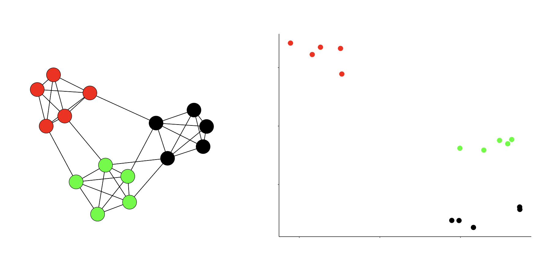
Imagine that at the center of each of these groups, there is a “group center”. Label these three points \(z_{\text{Black}}\), \(z_{\text{Green}}\) and \(z_{\text{Red}}\). We can estimate the number of edges between these three groups in a symmetric “probability matrix”, denoted by \(\hat P\). Then, by solving for the distances using the LS model, we see that

\[\hat d_{k,k'} = -\log\left(\frac{\hat P_{k,k'}}{E(\exp(\nu_i)^2)}\right)\]

where \(\hat d_{k,k'}\) is the estimated distance between points \(k\) and \(k'\) along the surface of \(\mathcal{M}^p(\kappa)\).